1. Introduction
When we talk about CNC machines, we usually think about machines that are commanded to move to certain locations and perform various tasks. In order to have an unified view of the machine space, and to make it fit the human point of view over 3D space, most of the machines (if not all) use a common coordinate system called the Cartesian Coordinate System.
The Cartesian Coordinate system is composed of three axes (X, Y, Z) each
perpendicular to the other two
[The word "axes" is also
commonly (and wrongly) used when talking about
CNC machines, and referring to the moving directions of the machine.]
.
When we talk about a G-code program (RS274/NGC) we talk about a number
of commands (G0, G1, etc.) which have positions as parameters (X- Y-
Z-). These positions refer exactly to Cartesian positions. Part of the
LinuxCNC motion controller is responsible for translating those positions
into positions which correspond to the machine
kinematics
[Kinematics: a two way function to
transform from Cartesian space to joint space.]
.
1.1. Joints vs Axes
A joint of a CNC machine is a one of the physical degrees of freedom of the machine. This might be linear (leadscrews) or rotary (rotary tables, robot arm joints). There can be any number of joints on a given machine. For example, one popular robot has 6 joints, and a typical simple milling machine has only 3.
There are certain machines where the joints are laid out to match kinematics axes (joint 0 along axis X, joint 1 along axis Y, joint 2 along axis Z), and these machines are called Cartesian machines (or machines with Trivial Kinematics). These are the most common machines used in milling, but are not very common in other domains of machine control (e.g. welding: puma-typed robots).
LinuxCNC supports axes with names: X Y Z A B C U V W. The X Y Z axes typically refer to the usual Cartesian coordinates. The A B C axes refer to rotational coordinates about the X Y Z axes respectively. The U V W axes refer to additional coordinates that are commonly made colinear to the X Y Z axes respectively.
2. Trivial Kinematics
The simplest machines are those in which which each joint is placed along one of the Cartesian axes. On these machines the mapping from Cartesian space (the G-code program) to the joint space (the actual actuators of the machine) is trivial. It is a simple 1:1 mapping:
pos->tran.x = joints[0];
pos->tran.y = joints[1];
pos->tran.z = joints[2];
In the above code snippet one can see how the mapping is done: the X position is identical with the joint 0, the Y position with joint 1, etc. The above refers to the direct kinematics (one direction of the transformation). The next code snippet refers to the inverse kinematics (or the inverse direction of the transformation):
joints[0] = pos->tran.x;
joints[1] = pos->tran.y;
joints[2] = pos->tran.z;
In LinuxCNC, the identity kinematics are implemented with the
trivkins kinematics module and extended to 9 axes. The default
relationships between axis coordinates and joint numbers are:
[If the machine (for example a lathe) is mounted with
only the X, Z and A axes and the INI file of LinuxCNC contains
only the definition of these 3 joints, then the previous assertion is false.
Because we currently have (joint0=X, joint1=Z, joint2=A) which
assumes that joint1=Y.
To make this work in LinuxCNC just define all the axes (XYZA),
LinuxCNC will then use a simple loop in HAL for unused Y axis.]
[Another way to make it work is to change the corresponding code and recompile the software.]
pos->tran.x = joints[0];
pos->tran.y = joints[1];
pos->tran.z = joints[2];
pos->a      = joints[3];
pos->b      = joints[4];
pos->c      = joints[5];
pos->u      = joints[6];
pos->v      = joints[7];
pos->w      = joints[8];
Similarly, the default relationships for inverse kinematics for trivkins are:
joints[0] = pos->tran.x;
joints[1] = pos->tran.y;
joints[2] = pos->tran.z;
joints[3] = pos->a;
joints[4] = pos->b;
joints[5] = pos->c;
joints[6] = pos->u;
joints[7] = pos->v;
joints[8] = pos->w;
It is straightforward to do the transformation for a trivial "kins" (trivkins kinematics) or Cartesian machine provided that there are no omissions in the axis letters used.
It gets a bit more complicated if the machine is missing one or more of the axis letters. The problems of omitted axis letters is addressed by using the coordinates= module parameter with the trivkins module. Joint numbers are assigned consecutively to each coordinate specified. A lathe can be described with coordinates=xz The joint assignments will then be:
joints[0] = pos->tran.x
joints[1] = pos->tran.z
Use of the coordinates= parameter is recommended for configurations that omit
axis letters.
[ Historically, the trivkins module did not support the
coordinates= parameter so lathe configs were often configured as XYZ
machines. The unused Y axis was configured to 1) home immediately, 2) use a
simple loopback to connect its position command HAL pin to its position
feedback HAL pin, and 3) hidden in gui displays. Numerous sim configs use
these methods in order to share common HAL files.]
The trivkins kinematics module also allows the same coordinate to be specified for more than one joint. This feature can be useful on machines like a gantry having two independent motors for the y coordinate. Such a machine could use coordinates=xyyz resulting in joint assignments:
joints[0] = pos->tran.x
joints[1] = pos->tran.y
joints[2] = pos->tran.y
joints[3] = pos->tran.z
See the trivkins man pages for more information.
3. Non-trivial kinematics
There can be quite a few types of machine setups (robots: puma, scara; hexapods etc.). Each of them is set up using linear and rotary joints. These joints don’t usually match with the Cartesian coordinates, therefore we need a kinematics function which does the conversion (actually 2 functions: forward and inverse kinematics function).
To illustrate the above, we will analyze a simple kinematics called bipod (a simplified version of the tripod, which is a simplified version of the hexapod).
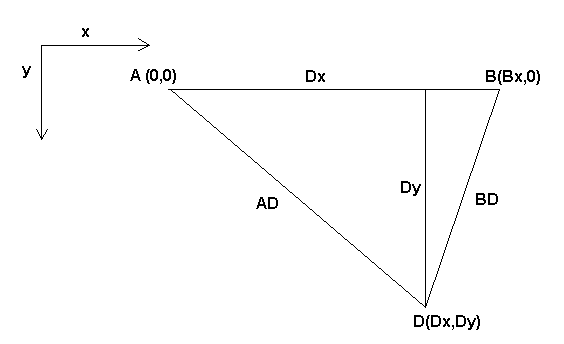
The Bipod we are talking about is a device that consists of 2 motors placed on a wall, from which a device is hung using some wire. The joints in this case are the distances from the motors to the device (named AD and BD in the figure).
The position of the motors is fixed by convention. Motor A is in (0,0), which means that its X coordinate is 0, and its Y coordinate is also 0. Motor B is placed in (Bx, 0), which means that its X coordinate is Bx.
Our tooltip will be in point D which gets defined by the distances AD and BD, and by the Cartesian coordinates Dx, Dy.
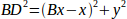
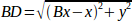
The job of the kinematics is to transform from joint lengths (AD, BD) to Cartesian coordinates (Dx, Dy) and vice-versa.
3.1. Forward transformation
To transform from joint space into Cartesian space we will use some trigonometry rules (the right triangles determined by the points (0,0), (Dx,0), (Dx,Dy) and the triangle (Dx,0), (Bx,0) and (Dx,Dy)).
We can easily see that:

likewise:
If we subtract one from the other we will get:

and therefore:
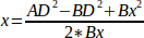
From there we calculate:

Note that the calculation for y involves the square root of a difference, which may not result in a real number. If there is no single Cartesian coordinate for this joint position, then the position is said to be a singularity. In this case, the forward kinematics return -1.
Translated to actual code:
double AD2 = joints[0] * joints[0];
double BD2 = joints[1] * joints[1];
double x = (AD2 - BD2 + Bx * Bx) / (2 * Bx);
double y2 = AD2 - x * x;
if(y2 < 0) return -1;
pos->tran.x = x;
pos->tran.y = sqrt(y2);
return 0;
3.2. Inverse transformation
The inverse kinematics is much easier in our example, as we can write it directly:

or translated to actual code:
double x2 = pos->tran.x * pos->tran.x;
double y2 = pos->tran.y * pos->tran.y;
joints[0] = sqrt(x2 + y2);
joints[1] = sqrt((Bx - pos->tran.x)*(Bx - pos->tran.x) + y2);
return 0;
4. Implementation details
A kinematics module is implemented as a HAL component, and is permitted to export pins and parameters. It consists of several "C" functions (as opposed to HAL functions):
int kinematicsForward(const double *joint, EmcPose *world,
const KINEMATICS_FORWARD_FLAGS *fflags,
KINEMATICS_INVERSE_FLAGS *iflags)
Implements the forward kinematics function.
int kinematicsInverse(const EmcPose * world, double *joints,
const KINEMATICS_INVERSE_FLAGS *iflags,
KINEMATICS_FORWARD_FLAGS *fflags)
Implements the inverse kinematics function.
KINEMATICS_TYPE kinematicsType(void)Returns the kinematics type identifier, típicamente KINEMATICS_BOTH:
-
KINEMATICS_IDENTITY (each joint number corresponds to an axis letter)
-
KINEMATICS_BOTH (forward and inverse kinematics functions are provided)
-
KINEMATICS_FORWARD_ONLY
-
KINEMATICS_INVERSE_ONLY
|
Note
|
GUIs may interpret KINEMATICS_IDENTITY to hide the distinctions between joint numbers and axis letters when in joint mode (typically prior to homing). |
int kinematicsSwitchable(void)
int kinematicsSwitch(int switchkins_type)
KINS_NOT_SWITCHABLE
The function kinematicsSwitchable() returns 1 if multiple kinematics types are supported. The function kinematicsSwitch() selects the kinematics type. See Switchable Kinematitcs.
|
Note
|
The majority of provided kinematics modules support a single kinematics type and use the directive "KINS_NOT_SWITCHABLE" to supply defaults for the required kinematicsSwitchable() and kinematicsSwitch() functions. |
int kinematicsHome(EmcPose *world, double *joint,
KINEMATICS_FORWARD_FLAGS *fflags,
KINEMATICS_INVERSE_FLAGS *iflags)
The home kinematics function sets all its arguments to their proper values at the known home position. When called, these should be set, when known, to initial values, e.g., from an INI file. If the home kinematics can accept arbitrary starting points, these initial values should be used.
int rtapi_app_main(void)
void rtapi_app_exit(void)
These are the standard setup and tear-down functions of RTAPI modules.
When they are contained in a single source file, kinematics modules may be compiled and installed by halcompile. See the halcompile(1) manpage or the HAL manual for more information.
4.1. Kinematics module using the userkins.comp template
Another way to create a custom kinematics module is to adapt the HAL component userkins. This template component can be modified locally by a user and can be built using halcompile.
See the userkins man pages for more information.
Note that to create switchable kinematic modules the required modifications are somewhat more complicated.
See millturn.comp as an example of a switchable kinematic module that was created using the userkins.comp template.