
1. 简介
Coordinated multi-axis CNC machine tools controlled with LinuxCNC, require a special kinematics component for each type of machine. This chapter describes some of the most popular 5-axis machine configurations and then develops the forward (from work to joint coordinates) and inverse (from joint to work) transformations in a general mathematical process for two types of machine.
The kinematics components are given as well as vismach simulation models to demonstrate their behaviour on a computer screen. Examples of HAL file data are also given.
Note that with these kinematics, the rotational axes move in the opposite direction of what the convention is. See section ["rotational axes"](https://linuxcnc.org/docs/html/gcode/machining-center.html#_rotational_axes) for details.
2. 5-Axis Machine Tool Configurations
In this section we deal with the typical 5-axis milling or router machines with five joints or degrees-of-freedom which are controlled in coordinated moves.
3-axis machine tools cannot change the tool orientation, so 5-axis machine tools use two extra axes to set the cutting tool in an appropriate orientation for efficient machining of freeform surfaces.
Typical 5-axis machine tool configurations are shown in Figs. 3, 5, 7 and 9-11 [1,2] in section Figures.
The kinematics of 5-axes machine tools are much simpler than that of 6-axis serial arm robots, since 3 of the axes are normally linear axes and only two are rotational axes.
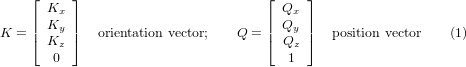
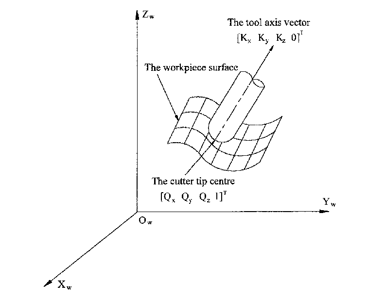
3. Tool Orientation and Location
CAD/CAM systems are typically used to generate the 3D CAD models of the workpiece as well as the CAM data for input to the CNC 5-axis machine. The tool or cutter location (CL) data, is composed of the cutter tip position and the cutter orientation relative to the workpiece coordinate system. Two vectors, as generated by most CAM systems and shown in Fig. 1, contain this information:
The K vector is equivalent to the 3rd vector from the pose matrix E6 that was used in the 6-axis robot kinematics [3] and the Q vector is equivalent to the 4th vector of E6. In MASTERCAM for example this information is contained in the intermediate output ".nci" file.
4. Translation and Rotation Matrices
Homogeneous transformations provide a simple way to describe the mathematics of multi-axis machine kinematics. A transformation of the space H is a 4x4 matrix and can represent translation and rotation transformations. Given a point x,y,x described by a vector u = {x,y,z,1}T, then its transformation v is represented by the matrix product

There are four fundamental transformation matrices on which 5-axis kinematics can be based:
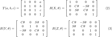
The matrix T(a,b,c) implies a translation in the X, Y, Z coordinate directions by the amounts a, b, c respectively. The R matrices imply rotations of the angle theta about the X, Y and Z coordinate axes respectively. The C and S symbols refer to cosine and sine functions respectively.
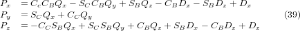
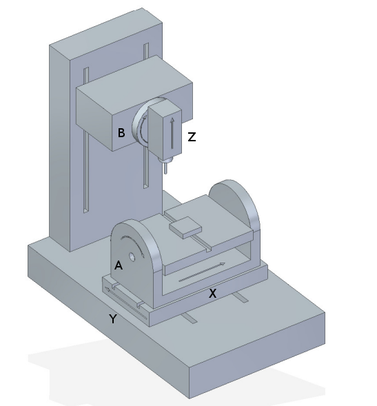
5. Table Rotary/Tilting 5-Axis Configurations
In these machine tools the two rotational axes mount on the work table of the machine. Two forms are typically used:
-
A rotary table which rotates about the vertical Z-axes (C-rotation, secondary) mounted on a tilting table which rotates about the X- or Y-axis (A- or B-rotation, primary). The workpiece is mounted on the rotary table.
-
A tilting table which rotates about the X- or Y-axis (A- or B-rotation, secondary) is mounted on a rotary table which rotates about the Z-axis (C-rotation, primary), with the workpiece on the tilting table.
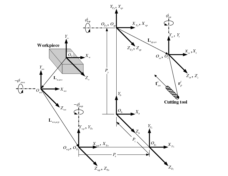
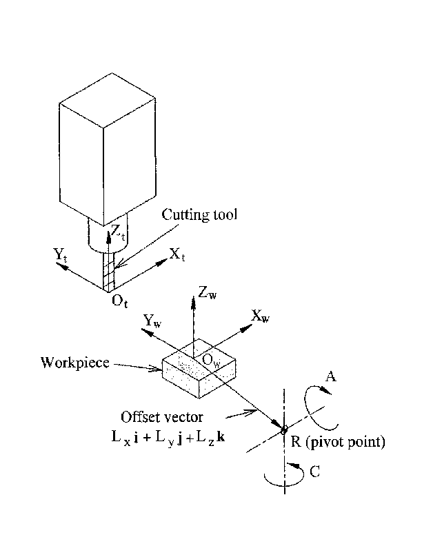
A multi-axis machine can be considered to consist of a series of links connected by joints. By embedding a coordinate frame in each link of the machine and using homogeneous transformations, we can describe the relative position and orientation between these coordinate frames
We need to describe a relationship between the workpiece coordinate system and the tool coordinate system. This can be defined by a transformation matrix wAt, which can be found by subsequent transformations between the different structural elements or links of the machine, each with its own defined coordinate system. In general such a transformation may look as follows:

where each matrix i-1Aj is a translation matrix T or a rotation matrix R of the form (2,3).
Matrix multiplication is a simple process in which the elements of each row of the lefthand matrix A is multiplied by the elements of each column of the righthand matrix B and summed to obtain an element in the result matrix C, ie.
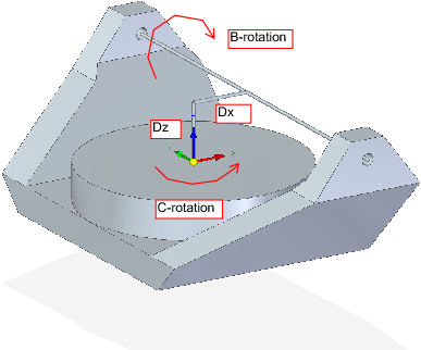
In Fig. 2 a generic configuration with coordinate systems is shown [4]. It includes table rotary/tilting axes as well as spindle rotary/tilting axes. Only two of the rotary axes are actually used in a machine tool.
First we will develop the transformations for the first type of configuration mentioned above, ie. a table tilting/rotary (trt) type with no rotating axis offsets. We may give it the name xyzac-trt configuration.
We also develop the transformations for the same type (xyzac-trt), but with rotating axis offsets.
Then we develop the transformations for a xyzbc-trt configuration with rotating axis offsets.
5.1. Transformations for a xyzac-trt machine tool with work offsets
We deal here with a simplified configuration in which the tilting axis and rotary axis intersects at a point called the pivot point as shown in Fig. 4. therefore the two coordinate systems Ows and Owp of Fig. 2 are coincident.
5.1.1. Forward transformation
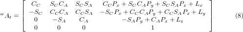
The transformation can be defined by the sequential multiplication of the matrices:

with the matrices built up as follows:
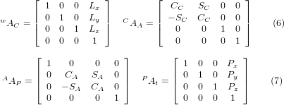
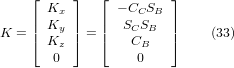
In these equations Lx, Ly, Lz defines the offsets of the pivot point of the two rotary axes A and C relative to the workpiece coordinate system origin. Furthermore, Px, Py, Pz are the relative distances of the pivot point to the cutter tip position, which can also be called the "joint coordinates" of the pivot point. The pivot point is at the intersection of the two rotary axes. The signs of the SA and SC terms are different to those in [2,3] since there the table rotations are negative relative to the workpiece coordinate axes (note that sin(-theta) = -sin(theta), cos(-theta) = cos(theta)).
When multiplied in accordance with (5), we obtain:
We can now equate the third column of this matrix with our given tool orientation vector K, ie.:
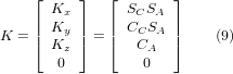
From these equations we can solve for the rotation angles thetaA, thetaC. From the third row we find:

and by dividing the first row by the second row we find:

These relationships are typically used in the CAM post-processor to convert the tool orientation vectors to rotation angles.
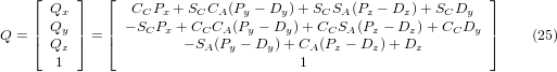
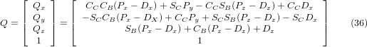
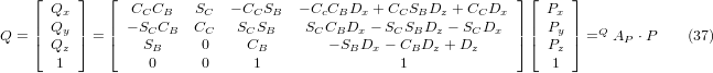
Equating the last column of (8) with the tool position vector Q, we can write:
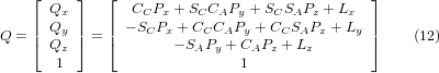
The vector on the right hand side can also be written as the product of a matrix and a vector resulting in:
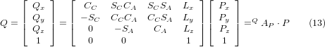
This can be expanded to give
which is the forward transformation of the kinematics.
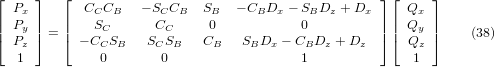
5.1.2. Inverse Transformation
We can solve for P from equation (13) as P = (QAP)-1 * Q. Noting that the square matrix is a homogeneous 4x4 matrix containing a rotation matrix R and translation vector q, for which the inverse can be written as:

where R^T is the transpose of R (rows and columns swappped). We therefore obtain:
The desired equations for the inverse transformation of the kinematics thus can be written as:
5.2. Transformations for a xyzac-trt machine with rotary axis offsets
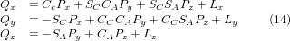
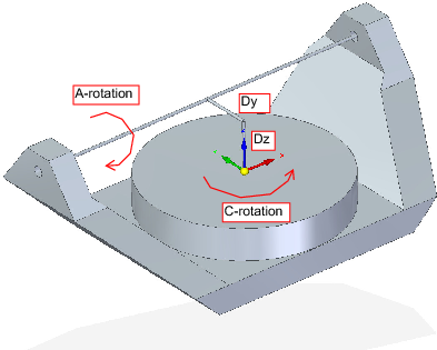
We deal here with a extended configuration in which the tilting axis and rotary axis do not intersect at a point but have an offset Dy. Furthermore, there is also an z-offset between the two coordinate systems Ows and Owp of Fig. 2, called Dz. A vismach model is shown in Fig. 5 and the offsets are shown in Fig. 6 (positive offsets in this example). To simplify the configuration, the offsets Lx, Ly, Lz of the previous case are not included. They are probably not necessary if one uses the G54 offsets in LinuxCNC by means of the "touch of" facility.
5.2.1. Forward Transformation
The transformation can be defined by the sequential multiplication of the matrices:

with the matrices built up as follows:
In these equations Dy, Dz defines the offsets of the pivot point of the rotary axes A relative to the workpiece coordinate system origin. Furthermore, Px, Py, Pz are the relative distances of the pivot point to the cutter tip position, which can also be called the "joint coordinates" of the pivot point. The pivot point is on the A rotary axis.
When multiplied in accordance with (18), we obtain:
We can now equate the third column of this matrix with our given tool orientation vector K, ie.:
From these equations we can solve for the rotation angles thetaA, thetaC. From the third row we find:

and by dividing the second row by the first row we find:

These relationships are typically used in the CAM post-processor to convert the tool orientation vectors to rotation angles.
Equating the last column of (21) with the tool position vector Q, we can write:
The vector on the right hand side can also be written as the product of a matrix and a vector resulting in:
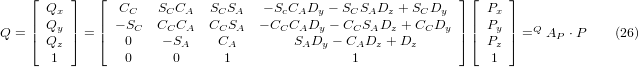
which is the forward transformation of the kinematics.
5.2.2. Inverse Transformation
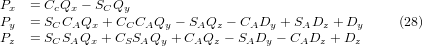
We can solve for P from equation (25) as P = (QAP)-1 * Q using (15) as before. We thereby obtain:
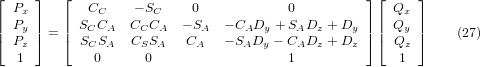
The desired equations for the inverse transformation of the kinematics thus can be written as:
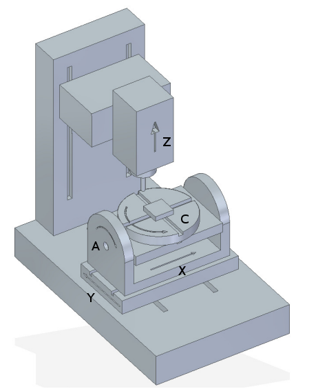
5.3. Transformations for a xyzbc-trt machine with rotary axis offsets
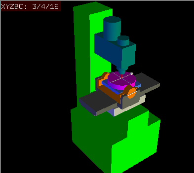
We deal here again with a extended configuration in which the tilting axis (about the y-axis) and rotary axis do not intersect at a point but have an offset Dx. Furthermore, there is also an z-offset between the two coordinate systems Ows and Owp of Fig. 2, called Dz. A vismach model is shown in Fig. 7 (negative offsets in this example) and the positive offsets are shown in Fig. 8.
5.3.1. Forward Transformation
The transformation can be defined by the sequential multiplication of the matrices:

with the matrices built up as follows:
In these equations Dx, Dz defines the offsets of the pivot point of the rotary axes B relative to the workpiece coordinate system origin. Furthermore, Px, Py, Pz are the relative distances of the pivot point to the cutter tip position, which can also be called the "joint coordinates" of the pivot point. The pivot point is on the B rotary axis.
When multiplied in accordance with (29), we obtain:
We can now equate the third column of this matrix with our given tool orientation vector K, i.e.:
From these equations we can solve for the rotation angles thetaB, thetaC. From the third row we find:

and by dividing the second row by the first row we find:

These relationships are typically used in the CAM post-processor to convert the tool orientation vectors to rotation angles.
Equating the last column of (32) with the tool position vector Q, we can write:
The vector on the right hand side can also be written as the product of a matrix and a vector resulting in:
which is the forward transformation of the kinematics.
5.3.2. Inverse Transformation
We can solve for P from equation (37) as P = (QAP)-1 * Q.
With the same approach as before, we obtain:
The desired equations for the inverse transformation of the kinematics thus can be written as:
6. Table Rotary/Tilting Examples
LinuxCNC includes kinematics modules for the xyzac-trt and xyzbc-trt topologies described in the mathematics detailed above. For interested users, the source code is available in the git tree in the src/emc/kinematics/ directory.
Example xyzac-trt and xyzbc-trt simulation configurations are located in the Sample Configurations (configs/sim/axis/vismach/5axis/table-rotary-tilting/) directory.
The example configurations include the required INI files and an examples subdirectory with G-code (NGC) files. These sim configurations invoke a realistic 3-dimensional model using the LinuxCNC vismach facility.
6.1. Vismach Simulation Models
Vismach is a library of python routines to display a dynamic simulation of a CNC machine on the PC screen. The python script for a particular machine is loaded in HAL and data passed by HAL pin connections. The non-realtime vismach model is loaded by a HAL command like:
loadusr -W xyzac-trt-guiand connections are made using HAL commands like:
net  :table-x   joint.0.pos-fb xyzac-trt-gui.table-x
net  :saddle-y  joint.1.pos-fb xyzac-trt-gui.saddle-y
...
See the simulation INI files for details of the HAL connections used for the vismach model.
6.2. Tool-Length Compensation
In order to use tools from a tool table sequentially with tool-length compensation applied automatically, a further Z-offset is required. For a tool that is longer than the "master" tool, which typically has a tool length of zero, LinuxCNC has a variable called "motion.tooloffset.z". If this variable is passed on to the kinematic component (and vismach python script), then the necessary additional Z-offset for a new tool can be accounted for by adding the component statement, for example:

The required HAL connection (for xyzac-trt) is:
net :tool-offset motion.tooloffset.z xyzac-trt-kins.tool-offsetwhere:
:tool-offset ---------------- signal name
motion.tooloffset.z --------- output HAL pin from LinuxCNC motion module
xyzac-trt-kins.tool-offset -- input  HAL pin to xyzac-trt-kins
7. Custom Kinematics Components
LinuxCNC implements kinematics using a HAL component that is loaded at startup of LinuxCNC. The most common kinematics module, trivkins, implements identity (trivial) kinematics where there is a one-to-one correspondence between an axis coordinate letter and a motor joint. Additional kinematics modules for more complex systems (including xyzac-trt and xyzbc-trt described above) are available.
See the kins manpage (\$ man kins) for brief descriptions of the available kinematics modules.
The kinematics modules provided by LinuxCNC are typically written in the C-language. Since a standard structure is used, creation of a custom kinematics module is facilitated by copying an existing source file to a user file with a new name, modifying it, and then installing.
Installation is done using halcompile:
sudo halcompile --install kinsname.c
where "kinsname" is the name you give to your component. The sudo prefix is required to install it and you will be asked for your root password. See the halcompile man page for more information (\$ man halcompile)
Once it is compiled and installed you can reference it in your config setup of your machine. This is done in the INI file of your config directory. For example, the common INI specificaion:
[KINS]
KINEMATICS = trivkins
is replaced by
[KINS]
KINEMATICS = kinsname
where "kinsname" is the name of your kins program. Additional HAL pins may be created by the module for variable configuration items such as the Dx, Dy, Dz, tool-offset used in the xyzac-trt kinematics module. These pins can be connected to a signal for dynamic control or set once with HAL connections like:
# set offset parameters
net :tool-offset motion.tooloffset.z xyzac-trt-kins.tool-offset
setp xyzac-trt-kins.y-offset 0
setp xyzac-trt-kins.z-offset 20
8. Figures
9. REFERENCES
-
AXIS MACHINE TOOLS: Kinematics and Vismach Implementation in LinuxCNC, RJ du Preez, SA-CNC-CLUB, April 7, 2016.
-
A Postprocessor Based on the Kinematics Model for General Five-Axis machine Tools: C-H She, R-S Lee, J Manufacturing Processes, V2 N2, 2000.
-
NC Post-processor for 5-axis milling of table-rotating/tilting type: YH Jung, DW Lee, JS Kim, HS Mok, J Materials Processing Technology,130-131 (2002) 641-646.
-
3D 6-DOF Serial Arm Robot Kinematics, RJ du Preez, SA-CNC-CLUB, Dec. 5, 2013.
-
Design of a generic five-axis postprocessor based on generalized kinematics model of machine tool: C-H She, C-C Chang, Int. J Machine Tools & Manufacture, 47 (2007) 537-545.