1. Introduction
When we talk about CNC machines, we usually think about machines that are commanded to move to certain locations and perform various tasks. In order to have an unified view of the machine space, and to make it fit the human point of view over 3D space, most of the machines (if not all) use a common coordinate system called the Cartesian Coordinate System.
The Cartesian Coordinate system is composed of three axes (X, Y, Z) each
perpendicular to the other two.
[The word “axes” is also
commonly (and wrongly) used when talking about
CNC machines, and referring to the moving directions of the machine.]
When we talk about a G-code program (RS274/NGC) we talk about a number
of commands (G0, G1, etc.) which have positions as parameters (X- Y-
Z-). These positions refer exactly to Cartesian positions. Part of the
LinuxCNC motion controller is responsible for translating those positions
into positions which correspond to the machine
kinematics.
[Kinematics: a two way function to
transform from Cartesian space to joint space]
1.1. Joints vs. Axes
A joint of a CNC machine is a one of the physical degrees of freedom of the machine. This might be linear (leadscrews) or rotary (rotary tables, robot arm joints). There can be any number of joints on a given machine. For example, one popular robot has 6 joints, and a typical simple milling machine has only 3.
There are certain machines where the joints are laid out to match kinematics axes (joint 0 along axis X, joint 1 along axis Y, joint 2 along axis Z), and these machines are called Cartesian machines (or machines with Trivial Kinematics). These are the most common machines used in milling, but are not very common in other domains of machine control (e.g. welding: puma-typed robots).
2. Trivial Kinematics
The simplest machines are those in which which each joint is placed along one of the Cartesian axes. On these machines the mapping from Cartesian space (the G-code program) to the joint space (the actual actuators of the machine) is trivial. It is a simple 1:1 mapping:
pos->tran.x = joints[0];
pos->tran.y = joints[1];
pos->tran.z = joints[2];
pos->a = joints[3];
pos->b = joints[4];
pos->c = joints[5];
In the above code snippet one can see how the mapping is done: the X position is identical with the joint 0, the Y posittion with with joint 1, etc. The above refers to the direct kinematics (one direction of the transformation). The next code snippet refers to the inverse kinematics (or the inverse direction of the transformation):
joints[0] = pos->tran.x;
joints[1] = pos->tran.y;
joints[2] = pos->tran.z;
joints[3] = pos->a;
joints[4] = pos->b;
joints[5] = pos->c;
As one can see, it’s pretty straightforward to do the transformation
for a trivial "kins" (kinematics) or Cartesian machine. It gets a bit more
complicated if the machine is missing one of the axes.
[If a
machine (e.g. a lathe) is set up with only the axes X,Z & A, and
the LinuxCNC inifile holds only these 3 joints defined, then the above
matching will be faulty. That is because we actually have (joint0=x,
joint1=Z, joint2=A) whereas the above assumes joint1=Y. To make it
easily work in LinuxCNC one needs to define all axes (XYZA), then use a
simple loopback in HAL for the unused Y axis.]
[One other
way of making it work, is by changing the matching code and
recompiling the software.]
3. Non-trivial kinematics
There can be quite a few types of machine setups (robots: puma, scara; hexapods etc.). Each of them is set up using linear and rotary joints. These joints don’t usually match with the Cartesian coordinates, therefore we need a kinematics function which does the conversion (actually 2 functions: forward and inverse kinematics function).
To illustrate the above, we will analyze a simple kinematics called bipod (a simplified version of the tripod, which is a simplified version of the hexapod).
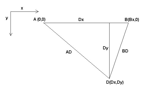
The Bipod we are talking about is a device that consists of 2 motors placed on a wall, from which a device is hung using some wire. The joints in this case are the distances from the motors to the device (named AD and BD in the figure).
The position of the motors is fixed by convention. Motor A is in (0,0), which means that its X coordinate is 0, and its Y coordinate is also 0. Motor B is placed in (Bx, 0), which means that its X coordinate is Bx.
Our tooltip will be in point D which gets defined by the distances AD and BD, and by the Cartesian coordinates Dx, Dy.
The job of the kinematics is to transform from joint lengths (AD, BD) to Cartesian coordinates (Dx, Dy) and vice-versa.
3.1. Forward transformation
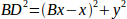
To transform from joint space into Cartesian space we will use some trigonometry rules (the right triangles determined by the points (0,0), (Dx,0), (Dx,Dy) and the triangle (Dx,0), (Bx,0) and (Dx,Dy).
We can easily see that
 ,
likewise
,
likewise
If we subtract one from the other we will get:

and therefore:
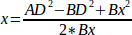
From there we calculate:

Note that the calculation for y involves the square root of a difference, which may not result in a real number. If there is no single Cartesian coordinate for this joint position, then the position is said to be a singularity. In this case, the forward kinematics return -1.
Translated to actual code:
double AD2 = joints[0] * joints[0];
double BD2 = joints[1] * joints[1];
double x = (AD2 - BD2 + Bx * Bx) / (2 * Bx);
double y2 = AD2 - x * x;
if(y2 < 0) return -1;
pos->tran.x = x;
pos->tran.y = sqrt(y2);
return 0;
3.2. Inverse transformation
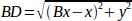
The inverse kinematics is lots easier in our example, as we can write it directly:

or translated to actual code:
double x2 = pos->tran.x * pos->tran.x;
double y2 = pos->tran.y * pos->tran.y;
joints[0] = sqrt(x2 + y2);
joints[1] = sqrt((Bx - pos->tran.x)*(Bx - pos->tran.x) + y2);
return 0;
4. Implementation details
A kinematics module is implemented as a HAL component, and is permitted to export pins and parameters. It consists of several “C” functions (as opposed to HAL functions):
int kinematicsForward(const double *joint, EmcPose *world,
const KINEMATICS_FORWARD_FLAGS *fflags,
KINEMATICS_INVERSE_FLAGS *iflags)
Implements the forward kinematics function.
int kinematicsInverse(const EmcPose * world, double *joints,
const KINEMATICS_INVERSE_FLAGS *iflags,
KINEMATICS_FORWARD_FLAGS *fflags)
Implements the inverse kinematics function.
KINEMATICS_TYPE kinematicsType(void)
Returns the kinematics type identifier, typically KINEMATICS_BOTH.
int kinematicsHome(EmcPose *world, double *joint,
KINEMATICS_FORWARD_FLAGS *fflags,
KINEMATICS_INVERSE_FLAGS *iflags)
The home kinematics function sets all its arguments to their proper values at the known home position. When called, these should be set, when known, to initial values, e.g., from an INI file. If the home kinematics can accept arbitrary starting points, these initial values should be used.
int rtapi_app_main(void)
void rtapi_app_exit(void)
These are the standard setup and tear-down functions of RTAPI modules.
When they are contained in a single source file, kinematics modules may be compiled and installed by comp. See the comp(1) manpage or the HAL manual for more information.